1. Laboratorio de Herpetología. Grupo de Investigación en Anfibios y Reptiles de la Facultad de Ciencias Exactas y Naturales y Agrimensura, Universidad Nacional del Nordeste (UNNE), Corrientes, Argentina.

2. Consejo Nacional de Investigaciones Científicas y Técnicas (CONICET).

* Autor de correspodencia: mringaramo@gamil.com

Recibido/Received: 30 de diciembre, 2026 | Aceptado/Acepted: 10 de junio, 2026 | Publicado/Published: 22 de junio, 2026

Como citar este artículo: Ingaramo, M. del R. & Marangoni, F. (2026). Determination of priority areas for amphibian conservation in the Iberá Natural Reserve and their relationship with existing conservation units. Revista FACENA 36(1), 81-109. Doi: https://doi.org/10.30972/fac.3619063

Resumen: La acelerada pérdida de biodiversidad impulsada por las actividades humanas resalta la necesidad de identificar Áreas Prioritarias para la Conservación (APC) de la Biodiversidad. La Reserva Natural Iberá (RNI) se ubica en la región centro-norte de la provincia de Corrientes y abarca un área de 13,000 km². Para implementar acciones de conservación, en 1994 se definieron cinco Unidades de Conservación (UC) con base en la infraestructura y la presencia de guardaparques, aunque los criterios utilizados para su selección no se explicaron con claridad. Los objetivos de este estudio fueron determinar Áreas Relevantes de Biodiversidad (ARB) de anfibios en la RNI para proponerlas como APC y evaluar la coincidencia de estas áreas con las actuales UC presentes en la reserva. Mediante muestreos de campo, revisión bibliográfica y de colecciones biológicas, se obtuvieron 1847 registros de 44 especies de anfibios para la RNI. La presencia/ausencia de especies se registró en cada una de las 28 cuadrículas en las que se dividió el área de estudio. Se calcularon la riqueza de especies, la diversidad filogenética y un índice combinado de biodiversidad, que incluye rareza y nivel de amenaza. Las ARB se identificaron mediante una condición denominada “máxima eficiencia”, para ello se realizaron búsquedas exactas (Complementariedad), obteniendo el mínimo conjunto de áreas que contuvieron a todas las especies, valores de diversidad filogenética e índice combinado de diversidad al menos una vez. La superficie mínima necesaria que representa a todas las especies de anfibios es de cinco cuadrículas (18%) y solo una coincide con una unidad de conservación actual. Se recomienda la adición de cuatro cuadrículas para cubrir los vacíos de conservación de anfibios. Esto proporciona un plan espacial para establecer nuevas áreas protegidas. Además, considerando los limitados recursos financieros destinados a la conservación en el área de estudio, estos resultados permiten una asignación rentable de recursos al dirigirse a los sitios más relevantes. El fortalecimiento de las medidas de protección en estas cinco áreas es fundamental como una herramienta de gestión estratégica para mitigar las extinciones locales de taxones amenazados.

Palabras claves: Anfibios; Conservación; Áreas protegidas; Iberá; Argentina.

Abstract: Accelerated biodiversity loss driven by human activities highlights the need to identify Priority Areas for Biodiversity Conservation (PABCSs). The Reserva Natural Iberá (RNI) is located in the central–northern region of Corrientes Province and covers an area of 13,000 km². To implement conservation actions, in 1994 five Conservation Units (CU) were defined and prioritized based on infrastructure and rangers presence, although the criteria used for their selection were not explained clearly enough. The objectives of this study were to identify Relevant Biodiversity Areas (RBA) for amphibians in the RNI in order to propose them as PABCSs, and to evaluate the spatial overlap between these areas and the current CUs within the reserve. A total of 1,847 records corresponding to 44 amphibian species were obtained for the RNI through field surveys, literature review, and examination of herpetological collections. Species presence/absence was recorded in each of the 28 grid cells into which the study area was divided. Species richness (S), phylogenetic diversity (PD), and a combined biodiversity index (CBI), including rarity and threat level, were calculated. RBAs were identified using an exact search approach (complementarity), obtaining the minimum set of areas that contained all species, phylogenetic diversity values, and CBI scores, a condition referred to as “maximum efficiency”. The minimum area required to represent all species comprised five grid cells (18%), of which only one overlapped with an existing CU. The addition of four grid cells is recommended to address current gaps in amphibian conservation. These findings provide a spatial blueprint for prioritizing land acquisition or the establishment of new protected areas. Furthermore, considering the limited financial and land resources allocated to conservation in the study area, these results allow for a cost-effective allocation of resources by targeting the most relevant sites of (PABCSs). Strengthening protection measures in these five areas is critical not just for species representation, but as a strategic management tool to mitigate local extinctions of threatened taxa.

Keywords: Amphibians; Conservation; Protected areas; Iberá; Argentina.

Introducción

Increasing anthropogenic pressures on biodiversity, particularly driven by high rates of land-use change and the overexploitation of natural resources, are leading to irreversible species loss and ecosystem degradation (Woodrofe, 2001 in Rodrigues et al., 2003). Identifying conservation priorities is therefore a strategic issue, given society’s strong dependence on the environmental services provided by ecosystems. Moreover, identifying the most threatened sites that harbor exceptional biodiversity is essential in order to conserve those components of evolutionary history embodied in the most vulnerable living organisms (Sechrest et al., 2002).

The establishment of protected areas (PA, hereafter), supported by a solid legal framework, represents a central strategy for biodiversity conservation. At present, protected areas enjoy increasing social acceptance, and society itself demands the expansion of land protection in regions of high biodiversity. However, current PAs systems are not always representative or effective, as many have been established in a biased manner in areas of low productive value (Toledo, 2005; Razola et al., 2006; Joppa and Pfaff, 2009). Therefore, it is essential to strengthen conservation systems through the incorporation of a diversified and complementary set of additional conservation instruments. Private reserves, biological corridors, land-use planning programs, economic incentives for sustainable production and ecological restoration extend biodiversity protection beyond the formal boundaries of protected areas and improve the assessment of existing PA networks (Koleff et al., 2009). These complementary approaches aim to ensure balanced ecosystem functioning, the sustained provision of ecosystem services, and the long-term persistence of the majority of species inhabiting these systems

The criteria commonly used for the selection of protected areas began to consolidate during the 1970s, incorporating conceptual contributions related to minimum area requirements, rarity, endemism, diversity, representativeness, irreplaceability, fragility, connectivity, ecosystem integrity, and vulnerability (Margules and Pressey, 2000; Lozano and Van Wyngaarden, 2005). The development and application of these criteria were based on the recognition that resources allocated to conservation are usually limited, thus requiring their optimal allocation. In this context, such analyses have provided a fundamental framework for guiding spatial prioritization and defining conservation funding strategies at multiple spatial scales (Vane-Wright et al., 1991; Pressey et al., 1993).

The “Esteros del Iberá” constitute one of the most important tropical wetland systems of the biosphere, in terms of both their spatial extent and the species they support. This complex ecosystem is composed of marshes, swamps, shallow lakes, and interconnected fluvial courses, covering approximately 13,000 km² in the northeastern and central regions of Corrientes Province, Argentina (Aranda, 2023).

The “Reserva Natural Iberá” (RNI, hereafter) was established in 1983 with the aim of conserving one of the largest and most important wetlands in South America. Since its creation, the reserve has undergone regulatory modifications, and currently the “Gran Parque Iberá” is located within its boundaries, encompassing an area of 768,000 hectares. This protected complex comprises 600,000 hectares of the Iberá Provincial Park and 168,000 hectares of the “Parque Nacional Iberá” (Fig. 1).

Neiff (1994) proposed the establishment of five Conservation Units (CU, hereafter) within the RNI (Fig. 1), as a compensatory measure for flooding associated with the “Yacyretá” Dam. These units were designated for strict protection through the installation of ranger stations and were selected to represent different Iberá landscape types, as well as their similarity to the current Paraná River valley in terms of species richness, distribution, and biotic abundance. However, as this proposal relied mainly on landscape-based criteria and on information available at the time, without an integrated quantitative assessment of biodiversity patterns, its effectiveness requires validation. Updated distributional data for previously unconsidered taxa are therefore essential to evaluate the representativeness of the CU system across the reserve.

Amphibians comprise a group of vertebrates that includes salamanders and newts (Urodela), caecilians (Gymnophiona), and frogs, toads, and horned frogs (Anura) (Cei, 1980). Their highest diversity occurs in tropical and subtropical regions, yet they represent a taxonomic group that is frequently overlooked in conservation policies. Amphibians exhibit a suite of morphological and ecological traits, such as ectothermy, a biphasic life cycle (aquatic–terrestrial), high skin permeability, strong site fidelity, and limited dispersal capacity, which make them particularly sensitive to environmental disturbances. In this context, amphibians are widely recognized as effective bioindicators of ecosystem condition, as their responses to physical, chemical, and biological changes are rapidly reflected in the composition, abundance, and structure of their communities (Blaustein and Wake, 1995; Wake and Vredenburg, 2008; Grant et al., 2016; Ficetola et al., 2019).

Recent studies have reinforced their importance in ecological monitoring and conservation, highlighting their increasing use in ecotoxicological assessments and biomonitoring programs due to their dual habitat use and physiological sensitivity (Mann et al., 2025). Moreover, amphibians are currently considered the most threatened vertebrate group globally, with approximately 40–41% of species at risk of extinction, mainly due to habitat loss, climate change, emerging diseases, pollution, and invasive species. Consequently, the study of amphibian diversity provides an integrated framework for assessing environmental quality and ecosystem integrity across both aquatic and terrestrial systems. In addition, amphibians play a key role in trophic networks, acting as both predators of invertebrates and prey for higher trophic levels, thereby contributing to ecosystem functioning. Spatial patterns of amphibian diversity have therefore become a valuable tool for guiding conservation strategies within an ecosystem-based approach, allowing the identification of priority areas and supporting more effective biodiversity management (Hocking and Babbitt, 2014; Borzée et al., 2025)

Within this framework, this study addresses two primary objectives. First, we identify Relevant Biodiversity Areas (RBAs) for amphibians within the RNI and propose them as priority areas for conservation (PABCSs). Second, we assess the degree of spatial overlap between them and the Conservation Units (CUs) currently established in the reserve. We hypothesize that the five existing CU do not adequately coincide with amphibian RBAs and therefore fail to effectively conserve the biodiversity of this group.

MATERIALS AND METHODS

Study area

The “Reserva Natural Iberá” (RNI) is located in the central–northern region of Corrientes Province, Argentina, and covers an area of approximately 13,000 km², or one-fifth of the total area of the province (Fig. 1). The study area comprises a complex of wetlands, including marshes, shallow lakes, swamps, and drainage channels, together with associated terrestrial environments such as “Pastizales de Lomada” and Paranaense, Chaco, and Espinal forests (Neiff, 2004). Within the ecoregional framework of Argentina, Iberá is recognized as a distinct ecological unit dominated by subtropical wetlands, with characteristic floristic, faunal, and functional attributes (Burkart et al., 1999). From a phytogeographic perspective, three major provinces converge within the RNI. To the west lies the Eastern District of the Chaco phytogeographic province, while to the east, from north to south, extend the “Distrito de los Campos” of the Paranaense province and the Espinillar or Ñandubay Districts of the Espinal province (Carnevali, 2003).The RNI includes five CUs: Galarza (200 km²), Iberá (100 km²), Itatí (130 km²), Yaguareté Corá (100 km²), and Camby Retá (100 km²), whose spatial distribution is shown in Figure 1.

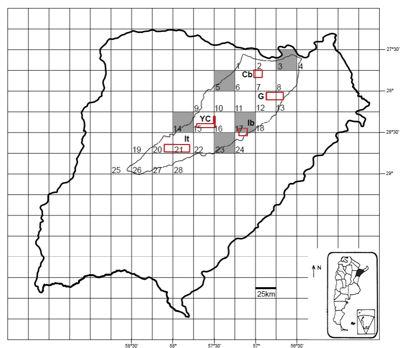
Figure 1. Study area. Reserva Natural Iberá (RNI) divided into 28 grid cells of 0.15° latitude–longitude. The red lines delimit the Conservation Units of the Reserva Natural Iberá, Corrientes Province, Argentina. Abbreviations of the CUs: Cb = Cambyretá, G = Galarza, Ib = Iberá, YC =Yaguareté-Corá, It = Itatí.

Data collection and analysis

For this study, we compiled a total of 1,847 amphibian records from our field surveys (285 records) and literature review (27 records). We also gathered an additional 1,535 records from herpetological collections at the Universidad Nacional del Nordeste (UNNEC), the Museo de La Plata (MLP), the Laboratorio de Genética Evolutiva of the Instituto de Biología Subtropical (CONICET–UNaM; LGE), and the Museo Argentino de Ciencias Naturales Bernardino Rivadavia (MACN). We conducted sampling primarily during the spring and summer months, when amphibians exhibit higher reproductive activity (vocalizations, amplexus, and egg laying), which facilitated observation and detection (Peltzer, 2006). We also performed additional sampling during the autumn and winter months to record species that remain active during these seasons, such as Boana pulchellus (Basso, 1990; Peltzer and Lajmanovich, 2007), among others (Table 1).

Table 1. Localities sampled in 21 seasonal surveys over six years (2007–2012). The sampling periods of each survey and the localities with their coordinates are presented below.

1.Localities and Coordinates: Colonia Carlos Pellegrini: -28.400000, -57.166667 | Ex obrador: -28.533333, -57.083333 | Pje. Galarza: -28.083333, -56.766667 | Ea. Santa Lucia Ñu: -28.066667, -56.650000 | Ea. San Lorenzo: -28.050000, -56.633333 | Ea. El Estribo: -28.500000, -57.083333 | Laguna Galarza: -28.100000, -56.683333 | Cadive cue: -28.083333, -56.566667 | Ea. Tataré: -28.033333, -56.600000 | Paraje Cambá Trapo: -28.500000, -56.983333 | Itá Corá: -28.883333, -58.166667 | Ea. San Juan miní: -28.350000, -57.816667 | San Miguel: -27.983333, -57.600000 | Loreto: -27.766667, -57.283333 | Ea. Tacuaralito: -27.733333, -57.166667 | Ea. San Juan Poriajú: -27.716667, -57.233333 | Ea. El Tránsito: -28.416667, -57.733333 | Ea. San Eugenio: -28.383333, -57.850000 | Ea. San Antonio: -28.783333, -58.333333 | Chavarría: -28.866667, -58.833333 | Ea. Iberá: -28.133333, -57.250000 | Pje. Uguay: -28.700000, -57.466667 | Ea. Rincón del Socorro: -28.400000, -57.350000 | Ea. Yacoví: -27.816667, -56.483333 | Ea. Rincón del Diablo: -28.733333, -58.033333 | Capitá Miní: -29.033333, -58.316667 | Ea. San Nicolás: -28.083333, -57.416667 | Laguna Fernández: -28.616667, -57.516667 | Ea. Curuzú Laurel: -27.466667, -57.016667 | Ea. San Alonso: -28.300000, -57.316667

2.Samples :1:January 20–25, 2007 | 2: March 29–April 4, 2007 | 3: June 23–28, 2007 | 4: August 25–30, 2007 | 5:October 27–31, 2007 | 6:December 26–30, 2007 | 7: March 27–31, 2008 | 8: April 27–30, 2008 | 9: August 1–8, 2008 | 10:October 26–31, 2008 | 11:December 19–22, 2008 | 12: April 23–27, 2009 | 13:September 29–October 2, 2009 / 2010 / 2011 | 14:November 15–20, 2009 | 15:February 26–March 6, 2010 | 16:September 27–October 2, 2010 | 17:December 6–10, 2010 | 18:February 4–12, 2011 | 19: August 24–September 2, 2011 | 20:November 21–24, 2011 | 21:February 12–17, 2012 |

We selected sampling sites based on their suitability for amphibian reproduction, including permanent and semi-permanent ponds, temporary pools, grasslands, marshes, drainage channels, and swamps (Fig. 2), in order to ensure comprehensive coverage of the habitats used by amphibians within the study area. During our field surveys, we conducted nocturnal site searches following the method proposed by Parris et al. (1999), as adapted by Peltzer et al. (2003), which combines Visual Encounter Surveys (Crump and Scott, 1994) and Audio Strip Transects (Zimmerman, 1994). We divided the RNI into 0.15° latitude–longitude grid cells (approximately 25 × 25 km) using Quantum GIS software, resulting in a total of 28 grid cells (Fig. 1). For each amphibian species, we recorded presence (1) or absence (0), considering at least one observation as equivalent to occupancy of the entire grid cell. This assumption is justified by the relatively large spatial resolution of the grid cells (approximately 25 × 25 km) and the sampling design, which combined nocturnal visual encounter surveys and acoustic transects across different habitat types within each cell. Given the environmental heterogeneity within grid cells, a confirmed record indicates the existence of suitable conditions for the species within that unit. Moreover, this approach is consistent with previous large-scale biodiversity assessments based on presence–absence data, where a single confirmed record is considered sufficient to assign species occurrence at the spatial resolution of analysis. While this may overestimate fine-scale occupancy, it provides a standardized and comparable framework for spatial and diversity analyses across the study area.

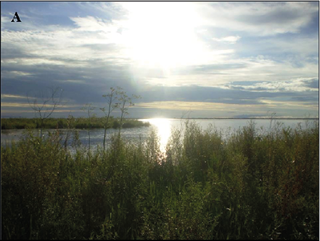
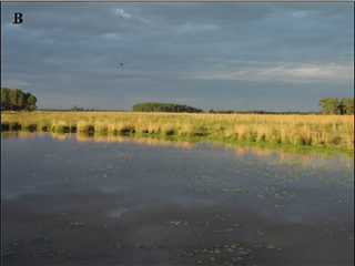
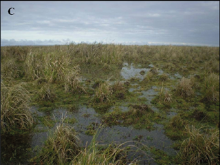
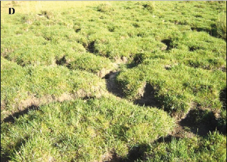
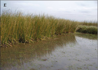
Figure 2. Studied habitats: Permanent pond (A), Semi-permanent pond (B), Temporary ponds (C), Grassland/malezal (D), Marshes, drainage channels, and swamps (E).

We applied and compared three indices that weigh different biodiversity attributes to identify RBA and propose them as PABCSs. First, we calculated species richness (S) as the total number of species present in each grid cell. Second, we assessed phylogenetic diversity (PD) using the index proposed by Vane-Wright et al. (1991). Third, we calculated a Combined Biodiversity Index (CBI), which incorporates species richness, rarity, and vulnerability (Rey Benayas and De la Montaña, 2003). We determined species vulnerability based on the most recent classification of Argentine amphibians (Vaira et al., 2012). We then assigned each category a score reflecting its degree of vulnerability: 1 for non-threatened species, 2 for data-deficient species, 3 for vulnerable species, 4 for threatened species, and 5 for endangered. This approach allowed us to integrate multiple facets of biodiversity to identify and prioritize areas for amphibian conservation.

Once we obtained the values of each index for every grid cell, we ranked them from highest to lowest and applied three comparative criteria. First, we selected as potential RBAs those grid cells with S, PD, and CBI values above 50% of the total sample. Second, we defined the top 15% of grid cells, following Burkart (2006), who proposed this minimum percentage of land necessary to protect biodiversity in Argentina. We applied a complementarity algorithm to each index following Colwell and Coddington (1994). In this framework, efficiency was defined as a measure of spatial optimization, referring to the identification of the minimum set of grid cells required to reach representation goals for all target species. By minimizing the total area while maximizing species coverage, the resulting Priority Areas for Biodiversity Conservation (PABCSs) ensure a cost-effective allocation of conservation efforts. We performed heuristic searches based on S, PD, and CBI using a stepwise procedure: first, the grid cell with the highest value was selected, and all species present in that cell were removed from the matrix. Using this reduced dataset, the next highest-ranking cell was selected and the process repeated—excluding already represented species—until all taxa were included (Vane-Wright et al., 1991). This same procedure was independently applied to PD and CBI.

Finally, we manually overlaid the maps of amphibian RBAs identified through complementarity with the RNI map, to assess the effectiveness of the five CUs currently established within the RNI.

RESULTS

A total of 1,847 records of 44 amphibian species were obtained across the 28 grid cells established for this study in the RNI (Appendix A). According to PD, the amphibian species with the highest phylogenetic value was Chthonerpeton indistinctum (W = 4.43), whereas the species with the lowest value was Rhinella diptycha (W = 1) (Table 2). In terms of the CBI a single species, Melanophryniscus cupreuscapularis, showed the highest value (CBI = 4), while three species (Leptodactylus luctator, Elachistocleis bicolor, and Scinax nasicus) exhibited the lowest values (CBI = 0.05) (Table 2).

Table 2. Phylogenetic diversity (PD) and combined biodiversity index (CBI) values for amphibian species recorded in the Reserva Natural Iberá. Species with the highest (+) and lowest (−) PD and CBI values are indicated in bold.

Criterion for retaining the top 50%

The distribution of amphibian RBA in the RNI, defined based on the criterion of retaining the top 50% of the total sample, was similar across the three indices, although the number of grid cells and their priority order differed (Fig. 3, Table 3). Ten RBA were identified according to S, while 11 RBA were determined based on PD and the CBI (Fig. 3, Table 3). The representational efficiency of the three indices was high; they were able to capture 100% of the amphibian species recorded in the reserve within the identified RBAs. This high level of species representativeness across all indices confirms their effectiveness in encompassing the total species diversity of the RNI (Table 3).

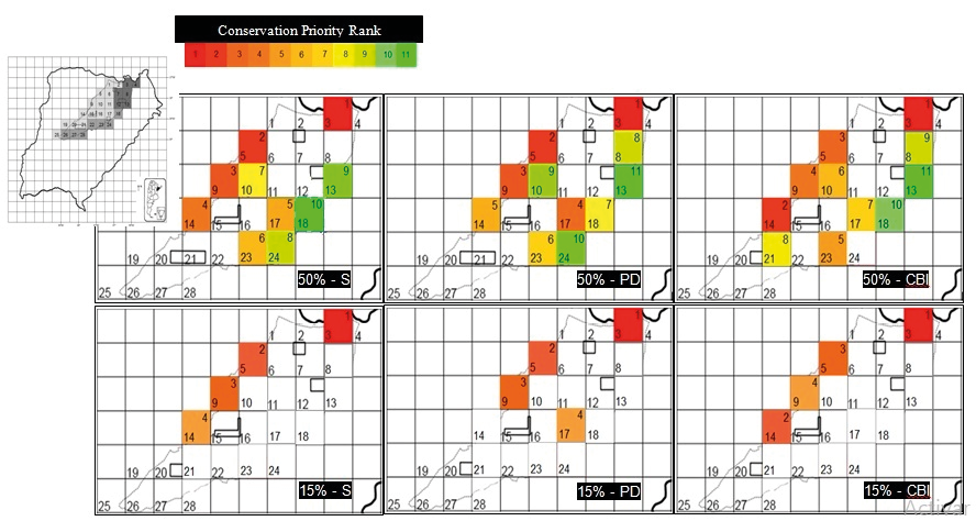
Figure 3. Relevant amphibian biodiversity conservation areas defined according to the criterion of conserving the top 50% or 15% based on species richness (S), phylogenetic diversity (PD), and the combined biodiversity index (CBI). In each grid cell, the top number indicates the conservation priority rank (1 = high priority to 11 = low priority), and the bottom number indicates the grid cell number (1 to 28).

Table 3. Conservation priority ranking of grid cells defined according to the top 50% criterion (A), top 15% criterion (B), and complementarity (C), based on species richness (S), phylogenetic diversity (PD) and combined biodiversity index (CBI). GCN = grid cell number. CR = cumulative richness. AE = added species.

Criterion for retaining the top 15%

The distribution of amphibian RBAs in the RNI, defined based on the criterion of retaining the top 15% of the total sample, identified four priority grid cells for conservation, with differences in their relative importance depending on the index used (Fig. 3, Table 3). For S and CBI, the same grid cells were selected, although their priority order differed, whereas for PD, the selection differed because this index excluded grid cell 14 and included grid cell 17 instead (Fig. 3, Table 3). In terms of efficiency regarding the total number of amphibian species included in the RBAs, S and CBI encompassed 42 of the 44 species recorded in the reserve, leaving out Chthonerpeton indistinctum and Leptodactylus mystacinus, while PD included 41 species, excluding Melanophryniscus cupreuscapularis, L. mystacinus, and Rhinella major.

Complementarity

The minimum area required to represent all amphibian species, according to the three calculated criteria, consisted of five grid cells, representing 18% of the total grid cells into which the RNI was divided (Table 3).

Based on S and CBI, the list of complementary grid cells differed only in the priority order of the last two, as each contributed only one new species. These species were Chthonerpeton indistinctum, present in grid cells 1, 8, 17, and 18, and Leptodactylus mystacinus, recorded in grid cells 21 and 23; therefore, either of these cells could serve as the final complementary grid cells (Table 3). PD produced a similar result, differing only in the priority order of the cells. Only the fifth complementary cell presented two possible alternatives, as both contributed the same value (Table 2).

Among the five grid cells identified as RBAs through complementarity based on S, PD, and CBI, only one grid (cell 17) overlapped with a Conservation Unit within the RNI (Fig 1). This minimal overlap highlights critical geographic gaps in the current reserve design, leaving major amphibian diversity hotspots entirely unprotected.

DISCUSSION

This study aimed to achieve two primary goals. First, we sought to identify Relevant Biodiversity Areas (RBAs) for amphibians within the RNI and proposed them as Priority Areas for Biodiversity Conservation (PABCSs). Second, we examined the spatial overlap between these RBAs and the Conservation Units (CUs) currently established within the reserve. The results indicate that using a combination of different indices to identify RBAs provides a more robust strategy than relying on a single criterion. In particular, simultaneously considering S, PD and CBI allowed the identification of grid cells that more comprehensively represent the amphibian diversity within the RNI. This approach avoids the bias that could arise from prioritizing only areas with high species richness, which do not capture phylogenetic variability or the vulnerability of amphibian species. These results are consistent with previous studies highlighting the importance of using multiple indices in systematic conservation planning, as selection based on a single parameter may lead to the protection of areas that share a high proportion of species, resulting in lower efficiency in terms of biological representativeness (Arzamendia and Giraudo, 2004; Ervin, 2003; Diniz-Filho et al., 2009). In this context, the application of multiple indices allowed the identification of complementary areas, thereby maximizing species coverage within a relatively limited area.

When applying the RBA selection criterion based on including grid cells with S, PD, and CBI values above the top 50% of the sample, the approach effectively ensured representation of all amphibian species recorded in the reserve. However, it incurred a high spatial cost, requiring roughly 53% of the total area to be allocated for conservation, which may be impractical from a land-use and management perspective. By contrast, adopting a criterion that preserves a minimum portion of the regional area, such as the 15% proposed by Burkart (2006), substantially reduced the area required and, consequently, the associated management costs. Nonetheless, this strategy did not guarantee the inclusion of all amphibian species in the RNI, highlighting a clear trade-off between biological completeness and operational feasibility in defining conservation priorities.

The five RBAs (grid cells 3, 5, 14, 17, and 23) identified using the complementarity algorithm encompassed a total area of 3,125 km², representing 18% of the 28 grid cells considered in the RNI. Among these, grid cell 3 contributed the highest complementary values of S, PD, and CBI. Its location in the northern part of the reserve, adjacent to the Paraná River and within the Paranaense phytogeographic province, supports high environmental heterogeneity, which accounts for the elevated amphibian diversity observed, including tropical-affinity species at the edge of their distribution (Manzano et al., 2004). Considering the rapid advance of forest exploitation and the construction and subsequent filling of the Yacyretá reservoir, which caused multiple impacts affecting populations in the northern reserve (Neiff and Poi de Neiff, 2006; Acerbi, 2005), it is crucial to strengthen protection measures in this grid cell and implement targeted conservation actions to ensure the persistence of the species inhabiting this area.

Grid cell 14 ranked second in conservation priority, as it contributed the highest number of complementary species under some threat category, including Melanophryniscus cupreuscapularis, a species with a restricted distribution in northwestern Corrientes and associated with habitats under strong anthropogenic pressure (Schaefer, 2007; Schaefer et al., 2012; Céspedez and Arias, 2014). Grid cell 5 was proposed as the third priority, complementing three additional species, two of which are considered rare (Dermatonotus muelleri and Leptodactylus elenae), resulting in a high CBI value.

Finally, grid cell 17 contributed Chthonerpeton indistinctum, a species categorized as Data- Deficient (Vaira et al., 2012), with aquatic habits and rare occurrences due to its unknown activity period throughout the year (Cajade, 2012). Grid cell 23 included Leptodactylus mystacinus, which was recorded only once within the RNI and does not present other notable conservation features.

When comparing the three criteria used to define RBAs (50%, 15%, and complementarity), the complementarity-based approach proved to be the most efficient for biodiversity conservation (Pressey et al., 1993; Williams et al., 1996; Williams, 1998; Reyers et al., 2000; Mondragón and Morrone, 2004; Arzamendia and Giraudo, 2004, 2012; Gil and Moreno, 2007). This approach enabled the protection of 100% of the amphibian species recorded in the RNI within a relatively small area, representing a critical advantage in contexts where financial resources and land available for conservation are limited.

The total area covered by the five Conservation Units (CUs) within the RNI was relatively small in relation to the reserve’s overall extent, encompassing approximately 66.000 ha, or only 5% of the total area. Furthermore, the results of this study indicated that the current configuration of these CUs may have limited representativeness and effectiveness for the comprehensive protection of the reserve’s amphibian fauna, as they overlapped with only a single grid cell (grid cell 17, corresponding to the Iberá CU) identified through the complementarity criterion. These findings therefore support our hypothesis that the current CUs in the RNI do not adequately align with the amphibian RBAs.

Chebez (2005) noted that the role of CUs in the studied area has been mainly administrative, primarily protecting plant communities in marshes, drainage channels, and swamps (Carnevali, 2003), while habitats such as “Lomadas Arenosas”, Espinal, grasslands, scrublands, and areas adjacent to the Paraná River remain largely unprotected. Similar shortcomings in the design and placement of protected areas have been reported in Santa Fe, Misiones, and northern Corrientes province (Giraudo, 2001; Arzamendia and Giraudo, 2004, 2012; Gil and Moreno, 2007; Etchepare et al., 2016). In the RNI, the current CUs show low overlap with the identified priority areas and limited representation of amphibian fauna, highlighting potential limitations of the current management system in ensuring long-term population viability.

In conclusion, our results underscore the importance of incorporating taxon-specific criteria, particularly for sensitive groups such as amphibians, into the design and planning of protected areas. The identification of Relevant Biodiversity Areas (RBAs) through the combined use of multiple indices and complementarity-based approaches provides a robust framework to strengthen the effectiveness of the Iberá conservation system. This approach not only ensures a more representative coverage of amphibian diversity but also promotes efficient allocation of limited conservation resources, supporting long-term preservation of regional biodiversity. Operationally, these identified RBAs should be integrated into future expansions of the Gran Parque Iberá or used to designate new core zones under strict enforcement, guiding private land easements and regional zoning updates.

CONFLICTS OF INTEREST

The authors declare no conflicts of interest.

ACKNOWLEDGMENTS

We sincerely thank the Consejo Nacional de Investigaciones Científicas y Técnicas (CONICET) and the Universidad Nacional del Nordeste (UNNE) for providing the necessary support and resources to carry out this research. We are grateful to Dr. Marcelo Beccaceci, Director of Recursos Naturales de la Provincia de Corrientes, for granting the required collection permits. We also acknowledge the staff of the Reserva Natural Iberá ranger station for their assistance, guidance, and support with fieldwork and logistics within the reserve. Special thanks to José Miguel Piñeiro for his contribution to map editing, and to Eduardo Etchepare, Victor Zaracho, José Luis Acosta, Camila Falcione, and Soledad Palomas for their invaluable help during the field surveys.

REFERENCES

Appendix A. Amphibians species richness at Reserva Natural del Iberá (RNI). Grids where the species is recorded. Source of data: C = collection. A = acoustic record. L1 = Álvarez et al., 2003. L2 = Fariña et al., 2014. L3 = Zaracho and Lavilla 2015.

REFERENCES

Acerbi, M. H. (2005). Los Esteros del Iberá amenazados. ¿Yacyretá culpable o inocente? En A. Brown, U. Martínez Ortiz, M. Acerbi, & J. Corcuera (Eds.), La situación ambiental Argentina 2005 (pp. 177–184). Fundación Vida Silvestre Argentina.
Álvarez, B., Aguirre, R., Céspedez, J., Hernando, A., & Tedesco, M. (٢٠٠٣). Herpetofauna del Iberá. En B. Álvarez (Ed.), Fauna del Iberá (pp. 99–178). EUDENE.
Aranda, M. D. (2023). Caracterización biogeográfica de los Esteros del Iberá. Bonplandia 32(2): 147–164.
Arzamendia, V. & Giraudo, A. R. (2004). Usando patrones de biodiversidad para la evaluación y diseño de áreas protegidas: las serpientes de la provincia de Santa Fe (Argentina) como ejemplo. Revista Chilena de Historia Natural, 77, 335–348.
Arzamendia, V., & Giraudo, A. R. (2012). A panbiogeographical model to prioritize areas for conservation along large rivers. Diversity and Distributions, 18, 168–179.
Basso, N. G. (1990). Estrategias adaptativas en una comunidad subtropical de anuros. Cuadernos de Herpetología. Serie Monografías Nº 1, 1–77.
Blaustein, A. R. & Wake, D. B. (1995). The puzzle of declining amphibian populations. Scientific American, 272, 52–57.
Borzée, A., Prasad, V. K., Neam, K., Tarrant, J., Kosch, T. A., Barata, I. M., Rais, M., Bickford, D., da Fonte, L. F. M., Wilcken, J., Ghosh, D., Mindje, M., Naik, H., Chanson, J., & Wren, S. (2025). Conservation priorities for global amphibian biodiversity. Nature Reviews Biodiversity, 1(12), 754–771.
Burkart, R., Bárbaro, N. O., Sánchez, R. O., & Gómez, D. A. (1999). Eco-regiones de la Argentina. Administración de Parques Nacionales.
Burkart, R. (2006). Las áreas protegidas de la Argentina. En A. Brown, U. Martínez Ortiz, M. Acerbi, & J. Corcuera (Eds.), La situación ambiental Argentina 2005 (pp. 399–404). Fundación Vida Silvestre Argentina.
Cajade, R. (2012). Chthonerpeton indistinctum (Reinhardt y Lütken, 1862). In Categorización del estado de conservación de la herpetofauna de la República Argentina. Ficha de los taxones. Anfibios. Cuadernos de Herpetología, 26, 163.
Carnevali, R. (2003). El Iberá y su Entorno Fitogeográfíco. EUDENE. 112p.
Cei, J. M. (1980). Amphibians of Argentina [Monografía]. Monitore Zoologico Italiano (Nuova Serie), Monograph 2, 1–609.
Céspedez, J. A. & Arias, A. M. (2014). Destruction of Type locality, new records and distribution of Melanophryniscus cupreuscapularis. FrogLog, 110, 63–65.
Chebez, J. C. (2005). Guía de las reservas naturales de la Argentina: Nordeste (Vol. 3). Editorial Albatros.
Colwell, R. K., & Coddington, J. A. (1994). Estimating terrestrial biodiversity through extrapolation. Philosophical Transactions of the Royal Society B: Biological Sciences, 345, 101–118.
Crump, M. L., & Scott, N. J. (1994). Visual encounter surveys. En W. R. Heyer, M. A. Donnelly, R. W. McDiarmid, L. C. Hayek, & M. S. Foster (Eds.), Measuring and monitoring biological diversity: Standard methods for amphibians (pp. 84–91). Smithsonian Institution Press.
Diniz-Filho, J. A. F., Bini, L. M., Rangel, T. F., Loyola, R. D., Hof, C., Nogués-Bravo, D., & Araújo, M. B. (2009). Partitioning and mapping uncertainties in ensembles of forecasts of species turnover under climate change. Ecography, 32(6), 897–906
Ervin, J. (2003). Rapid assessment of protected area management effectiveness in four countries. BioScience, 53, 833–841.
Etchepare, E. G., Giraudo, A. R., Arzamendia, V., Bellini, G. P., & Álvarez, B. B. (2016). Eficiencia de las unidades de conservación definidas en la Reserva Natural Iberá (Argentina) en la protección de la diversidad de reptiles. Iheringia. Serie Zoología, 107, e2017011.
Fariña, N. D., Villalba, O. E., Boeris, J. M., Krauczuk, E. R., Ferro, J. M. & Baldo, D. (2014). Nuevos registros de Leptodactylus furnarius Sazima & Bokermann 1978 (Anura: Leptodactylidae) en Argentina. Cuadernos de Herpetología, 28, 49–50.
Ficetola, G. F., Manenti, R., & Taberlet, P. (2019). Environmental DNA and metabarcoding for the study of amphibians and reptiles: Species distribution, the microbiome, and much more. Amphibia-Reptilia, 40(2), 129–148.
Gil, G., & Moreno, C. E. (2007). Los análisis de complementariedad aplicados a la selección de reservas de la biosfera: efecto de la escala. Monografías Tercer Milenio 6, 63–70.
Giraudo, A. R. (2001). Serpientes de la Selva Paranaense y del Chaco Húmedo. Taxonomía, biogeografía y conservación. LOLA.
Grant, E. H. C., Miller, D. A. W., Schmidt, B. R., Adams, M. J., Amburgey, S. M., Chambert, T., Grayson, K. L., Harris, R. N., Jackson, S., Richardson, J. L., Walls, S. C., White, L. A., & Muths, E. (2016). Quantitative evidence for the effects of multiple drivers on continental-scale amphibian declines. Scientific Reports, 6(1), 25625.
Hocking, D. J., & Babbitt, K. J. (2014). Amphibian contributions to ecosystem services. Herpetological Conservation and Biology, 9(1), 1–17.
Joppa, L. N., & Pfaff, A. (2009). High and far: biases in the location of protected areas. PloS One 4(12), e8273.
Koleff, P., Tambutti, M., March, I. J., Esquivel, R., Cantú, C., Lira-Noriega, A., & Urquiza-Haas, T. (2009). Identificación de prioridades y análisis de vacíos y omisiones en la conservación de la biodiversidad de México. In J. S. Sarukhán, R. Dirzo, R. González, & I. J. March (Eds.), Capital natural de México (Vol. 2, pp. 651–718). Comisión Nacional para el Conocimiento y Uso de la Biodiversidad (CONABIO).
Lozano, M. T. F., & Van Wyngaarden, W. (2005). Prioridades de conservación biológica para Colombia. Sociedad Misionera CSA.
Mann, R., Gust, K. A., Mayfield, D. B., & Ludwigs, J. D. (2025). Key challenges and advancements in amphibian ecotoxicological assessments and biomonitoring programs. Environmental Toxicology and Chemistry, 44(3), 658–673.
Manzano, A. S., Baldo, D., & Barg, M. (2004). Anfibios del Litoral Fluvial Argentino. Temas de la Biodiversidad del Litoral fluvial argentino INSUGEO, Miscelánea, 12, 271–290.
Margules, C. R., & Pressey, R. L. (2000). Systematic conservation planning. Nature 405, 243–253.
Méndez Iglesias, M. (2003). Avances en los métodos para la selección de reservas naturales ornitológicas. El Draque, 4, 243–257.
Mondragón, E. A., & Morrone, J. J. (2004). Propuesta de áreas para la conservación de aves de México, empleando herramientas panbiogeográficas e índices de complementariedad. Interciencia, 29, 112–120.
Neiff, J. J. (1994). Ambientes protegidos y áreas compensatorias del embalse de Yaciretá. Presentado al Superior Gobierno de la Provincia de Corrientes, Subsecretaría de Recursos Naturales y Medio Ambiente.
Neiff, J. J. (2004). El Iberá… ¿en peligro? Fundación Vida Silvestre de Argentina.
Neiff, J. J., & Poi de Neiff, A. (2006). Situación ambiental en la ecorregión Iberá. En A. Brown, U. Martinez Ortiz, M. Acerbi, & J. Corcuera (Eds.), La situación ambiental argentina 2005 (pp. 177–184). Fundación Vida Silvestre Argentina.
Parris, K. M., Norton, T.W., & Cunningham, R. B. (1999). A comparison of techniques for sampling amphibians in the forests of South–East Queensland, Australia. Herpetologica 55:271–283.
Peltzer, P. M. (2006). La fragmentación de hábitat y su influencia en la diversidad y distribución de anfibios anuros de áreas ecotonales de los dominios fitogeográficos amazónico y chaqueño [Tesis de doctorado, Universidad Nacional de La Plata, Facultad de Ciencias Naturales y Museo].
Peltzer, P. M., Lajmanovich, R. C. & Beltzer, A. H. (2003). The effects of habitat fragmentation on amphibian species richness in the floodplain of the middle Paraná River. Herpetological Journal, 13, 95–98.
Peltzer, P. M., & Lajmanovich, R. C. (2007). Amphibians. In M. H. Iriondo, J. C. Paggi, & M. J. Parma (Eds.), The Middle Paraná River: Limnology of a subtropical wetland (pp. 327–340). Springer.
Pressey, R. L., Humphries, C. J., Margules, C. R., Vane–Wright, R. I., & Williams, P. H. (1993). Beyond opportunism: key principles for systematic reserve selection. Trends in Ecology and Evolution, 8, 124–128.
Razola, I., Rey Benayas, J. M., De la Montaña, E., & Cayuela, L. (2006). Selección de áreas relevantes para la conservación de la biodiversidad. Ecosistemas, 15, 34–41.
Rey Benayas J. M., & De La Montaña, E. (2003). Identifying areas of high-value vertebrate diversity for strengthening conservation. Biological Conservation, 114, 357–370.
Reyers, B., Van Jaarsveld, A. S., & Krüger, M. (2000). Complementarity as a biodiversity indicator strategy. Proceedings of the Royal Society of London B: Biological Sciences, 267, 505–513.
Rodrigues, A. S. L.; Tratt, R.; Wheeler, B. D., & Gaston, K. J. (2003). The performance of existing networks of conservation areas in representing biodiversity. Proceedings of the Royal Society of London B: Biological Sciences 266(1427), 1453–1460.
Schaefer, E. F. (2007). Restricciones cuantitativas asociadas con los modos reproductivos de los anfibios en áreas de impacto por la actividad arrocera en la provincia de Corrientes [Tesis de doctorado, Universidad Nacional de La Plata, Facultad de Ciencias Naturales y Museo].
Schaefer, E. F., Duré, M. I., & Céspedez, J. A. (2012). Melanophryniscus cupreuscapularis (Céspedez & Álvarez, 2000). In Categorización del estado de conservación de la herpetofauna de la República Argentina. Ficha de los taxones. Anfibios. Cuadernos de Herpetología, 26, 165.
Sechrest, W., Brooks, T. M., da Fonseca, G. A., Konstant, W. R., Mittermeier, R. A., Purvis, A., & Gittleman, J. L. (2002). Hotspots and the conservation of evolutionary history. Proceedings of the National Academy of Sciences, 99(4), 2067–2071.
Toledo, V. M. (2005). Repensar la conservación: ¿áreas naturales protegidas o estrategia bioregional. Gaceta ecológica, 77, 67–83.
Vaira, M.; Akmentins, M.; Attademo, A.; Baldo, D.; Barrasso, D.; Barrionuevo, S.; Basso, N.; Blotto, B.; Cairo, S.; Cajade, R.; Céspedez, J.; Corbalán, V.; Chilote, P.; Duré, M.; Falcione, C.; Ferraro, D.; Gutierrez, F.G.; Ingaramo, M.R.; Junges, C.; Lajmanovich, R.; Lescano, J.N.; Marangoni, F.; Martinazzo, L.; Marti, R.; Moreno, L.; Natale, G.S.; Pérez Iglesias, J.M.; Peltzer, P.; Quiroga, L.; Rosset, S.; Sanabria, E.; Sanchez, L.; Schaefer, E.; Úbeda, C. & Zaracho, V. (2012). Categorización del estado de conservación de los anfibios de la República Argentina. Cuadernos de Herpetología, 26, 131–159.
Vane–Wright, R. I., Humphries, C. I. & Williams, P. H. (1991). What to protect? Systematics and the agony of choice. Biological Conservation, 55, 235–254.
Wake, D. B., & Vredenburg, V. T. (2008). Are we in the midst of the sixth mass extinction? A view from the world of amphibians. Proceedings of the National Academy of Sciences, 105(supplement_1), 11466–11473.
Williams, P. H. (1998). Key sites for conservation: Area selection methods for biodiversity. En G. M. Mace, A. Balmford, & J. R. Ginsberg (Eds.), Conservation in a changing world: Integrating processes into priorities for action (pp. 211–249). Cambridge University Press.
Williams, P., Gibbons, D., Margules, C., Rebelo, A., Humphries, C. & Pressey, R. (1996). A Comparison of Richness Hotspots, Rarity Hotspots, and Complementary Areas for Conserving Diversity of British Birds. Conservation Biology, 10, 155–174.
Woodruff, D. S. (2001). Declines of biomes and biotas and the future of evolution. Proceedings of the National Academy of Sciences, 98(10), 5471–5476.
Zaracho, V. H., & Lavilla, E. O. (2015). Diversidad, distribución espacio-temporal y turnos de vocalización de anuros (Amphibia, Anura) en un área ecotonal del nordeste de Argentina. Iheringia. Serie Zoología, 105(2), 199–208.
Zimmerman, B. L. (1994). Audio strip transects. In W. R. Heyer, M. A. Donnelly, R. W. McDiarmid, L. C. Hayek, & M. S. Foster (Eds.), Measuring and monitoring biological diversity: Standard methods for amphibians (pp. 92–97). Smithsonian Institution Press.